Multiple Regression is similar to Trend (Linear) Regression except with more Xs, or Independent Variables. Often, the Y or Dependent Variable can be explained by more than one Independent Variable. For example, you may have sales data that is dependent on many factors: time of year, advertising dollars spent, and/or special promotions implemented. Each of these factors potentially has an influence over the sales figures. Multiple Regression is one Forecasting technique that determines the Independent Variable with the greatest impact. As with Trend (Linear) Regression, Multiple Regression must be interpreted and evaluated by the individual performing the Forecast. There are accuracy and descriptive statistics that help explain what is implied and predicted by the Multiple Regression Forecast.
Like Trend (Linear) Regression, the slope coefficients, such as m, needs to be interpreted. The coefficients represent the change in Y, or the Dependent Variable, from a change in the X, or Independent Variable, of interest. Multiple Regression determines how more than one Independent Variable influences a single Dependent Variable.
To use the Multiple Regression Forecasting technique:
- Click on
 and open the ForecastingExamples.xls file.
Note: The ForecastingExamples.xls file is a data example to demonstrate how the Multiple Regression method is used. For your company’s purposes, you will have your own data available. - Click on the Multiple Regression sheet.
The spreadsheet contains 56quarters covering 1993Q1 through 2006Q4. The raw sales numbers act as the dependent variable. Additionally, the following independent variables are included:
Variable Description TIME Index of Time
TIME(2) Index of Time Squared (accounts for nonlinearity) Q2 - Q4 Seasonal Dummy variable to account for seasonality in Q2, Q3 and Q4.
SP500 Standard & Poor’s 500 Stock Index - Click in a cell containing data and open ForecastX by clicking on
 . The Data capture window is displayed. Notice that ForecastX selects the relevant data from your spreadsheet and determines that it is in columns and arranged in quarters.
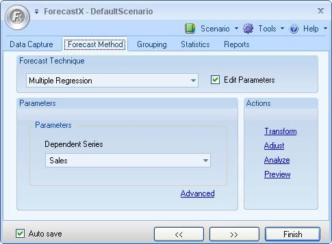
 - Click on the Forecast Method tab, and from the forecasting Technique drop down list, select Multiple Regression. The Multiple Regression Forecasting technique displays.

- Select Edit parameters to activate Multiple Regression’s parameters. ForecastX automatically selects which series in the data is the dependent series. If you would like to use a different series, select another series from the dropdown list.
- On the Reports tab, select Audit Trail Ensure that all other reports are not selected.
- Select Fitted Values Table from the Audit Trail report tab to compare the actual values with the Forecasted values.
- Click Finish.
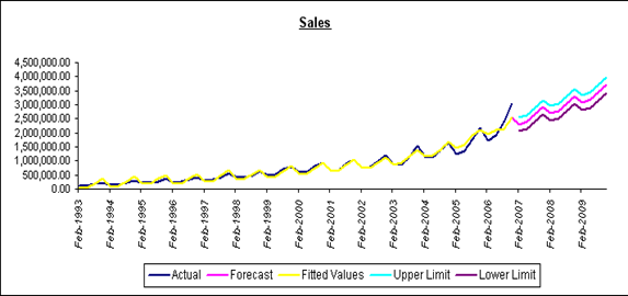
ForecastX has provided you with a detailed report of your Multiple Regression forecast that includes a graph, a fitted values table, an ANOVA chart, and a Coefficient Table.

The summary contents of the forecast and the values table are included in the ForecastX Audit Trail REport. The MAPE is 16.45%, while the R-Squared value is 96.59.

These values indicate you can have a high degree of confidence in the forecast. As you scroll down through the Audit Trail report, you can view the fitted values compared to the actual values at each data point.
The Audit Trail report in ForecastX is a powerful feature that enabled you to view all the relevant statistics when deciding whether to trust your forecast. In this case, for your Multiple Regression forecast, you can see that ForecastX included each independent series in the model. Additionally, ForecastX calculated the F-Test and T-test for each independent series. This enables you to decide objectively which series has the greatest influence on your dependent series, Sales. From the T-Test, you can see that Q4 is the independent series with the greatest influence on the Sales balance.